COSMOS - Stars, Sight and Science 2005
Star Clusters Project: Write-Up for Future Advisors
Open Clusters: Becca Gallery, Jared Rosen, and Molly Zimmerman Advised by Laura Chomiuk
Globular Clusters: Amanda Loo and Catherine Russell Advised by
Kirsten Howley


Day 1 for Laura: Outline of discussion (in pdf) about "What is a star?"
and Why
are star clusters interesting?". Introduction to Hydrostatic Equilibrium, Fusion, etc.
Day 1 for Kirsten: A powerpoint lecture on the physics and
history of "What is a star?"

Day 2: Stellar Evolution Powerpoint Lecture. Kirsten and Laura's
Groups merge to hear a lecture from Kirsten on stellar evolution.
We also did some fun demos!
Ideal Gas Law at Constant Pressure: Immerse a balloon in
liquid nitrogen to watch it shrink. Hilary's husband Greg was kind enough to supply the cold stuff.


Room-Temperature, Inflated Balloon
Is that Kirsten's icy stare deflating the balloon? Or is it...Liquid Nitrogen???
Ideal Gas Law at Constant Volume: Can Crushing! Boil a
bit of water in a pop can to fill it with steam, then immerse the can in water and watch it collapse!

No, that can's not being crushed by the
strength of Laura's grip...it's the Ideal Gas Law!!
An interactive
applet illustrating the Ideal Gas Law.

Day 3: Balloon H-R Diagram. We supplied the students with sturdy foam board, big party balloons, smaller
water balloons, markers, and
tape. We instructed them to create their own H-R diagram, using the appropriate sizes and colors of balloons.
Tips:
1) Water balloons are REALLY hard to blow up. I wouldn't use those next time.
2) The students sort of had a tendency to copy their diagrams from figures in their notes. I would consider not letting them use their
notes, in order to force them to think things through. Still debating on that one.


The sweat of Jared's lungs (Open Cluster Group)
Team Globular Cluster's HR Diagram

Observing:
Globular cluster people observed M5 (for a pretty picture) and M13 (for a pretty pic and a CMD). The open cluster group
observed M11 and NGC 6819. They observed two clusters to observe what changes in data between clusters of significantly different ages.
We observed in B,V,R. We intended to use only B and V images for our CMDs-- R is needed for three-color images. CMDs made with B and V
seem to work just fine.
"Long" exposures tended to be between 70 and 120 seconds, as hinted at by the NOAO
exposure time calculator. These exposure times gave reasonable results. However, we had originally planned to run daophot on multiple
long exposures, and average the results. Unfortunately, daophot can be grueling, and our students did not have time to reduce multiple
images, so our photometry was not as deep as it could be. We would suggest a bit longer exposures next year-- perhaps several
2-3 minute
exposures.
"Short" exposures were between 15 and 20 seconds. These served well to give photometry of the brightest stars in the frame.
We also observed a standard star, HD 338808. 5 second exposures in all filters worked well for this star. One should also note the
existence of Stetson standard stars. These are standard stars in bright star
clusters-- including M11 and M13! There are hundreds of standard stars in each cluster. These should be very useful. We just decided not
to use them this year because we had no way of easily transforming between ra/dec and CCD pixel coordinates for the standard stars.
Are Kirsten and Laura fancy enough to scan in their log sheets?

Late-Night Open Cluster Party
Kirsten, do you have a photo of your group observing that you want to include?

3-Color Images:
Pretty 3-color images are really easy to make, as long as you have decent images in B, V, and R (or any three filters!)
We suggest using DS9-- it's really simple and intuitive, and has the added bonus that DS9 is the tool astronomers actually
use!
We just downloaded the newest version of DS9 and made an RGB image in under 5 minutes. You can too! Easy step by step
directions:
1) Calculate shifts between your three images. Shifts greater than 1 pixel or so will be evident in your images, and we don't
want that. We had our students measure the shifts. They picked the same five stars or so in each band (one in each corner, and
one in the center) and measured the centroid of each using IRAF imexam ('r' command). Then, they calculated the shift from
band to band for each star. Finally, they averaged all the shifts for the stars, and used this as their final shift.
2) Now, if DS9 behaved itself and didn't try to be too smart, you could just apply the shifts you've found using IRAF imshift.
However, as Kirsten learned the hard way, imshift neglects to put some crucial information in the shifted image's header, so
when you display it with DS9, the image is not shifted at all. So, what we would suggest is, shift your image with a simple
program in IDL which removes the header. Of use imshift, but then delete the header. Be creative! But test your method before
showing it to the students.
3) See if you have the newest version of DS9, on your relevant computer. The easiest way to do this is start up DS9 like usual,
click on "Frame" up at the top, and see if directly under "New Frame" it lists "New Frame RGB". If it does, skip to step 4. If
it doesn't, then you need to download the newest version.
4) Download DS9. Don't worry! This is really really easy. DS9 is apparently
just one file. So no scary libraries, paths, etc. Simply go and download DS9 3.0.3 for your operating system. Apparently this
works for Windows machines, too! After you download it, you basically just need to unzip it (on a mac, double-click on the .gz
file, and your mac will unpack it for you. A DS9 icon will appear there, on your Desktop. i'm not sure exactly what to do on
the other operating systems, but i bet it's easy!)
5) Open up DS9. On my mac, I just clicked on the DS9 icon that appeared on my desktop.
6) Now, go click on Frame at the top, and then click on "New Frame RGB". A
little window should appear that says Red, Green, Blue in it, and has some
red squares. Don't close this, this is your control panel!!
FYI--In this control panel, there are two columns-- "Current" and "View". You can only have R, G, OR B selected under Current.
Whichever one is selected is the color you currently have control over. If you load an image, it will appear in that color. You
can only change the stretch/contrast on that image that is selected. Under the "View" column, you can have any number of frames
selected. These are the colors that are actually showing on the screen.
7) So-- let's say you wanted to load your R filter image first. Make sure "Red" is selected under Current. Back in the main DS9
window, click on "File" at the top, and then "Open". Find your R image and load it up. Of course, your images should be .fits.
When you've loaded it, go back to the top of the main window, and click on "Scale". Click on "Scale Parameters", and pick some
reasonable Min/Max values. Also under "Scale", you can pick if you want your image displayed on a Linear or Logarithmic scale,
etc.
Also, Click on "Edit" and then "Colorbar". This will allow you to change the stretch/contrast of your image display by dragging
your mouse around the image area, while holding down the left mouse button (or your one mouse button, on a powerbook)
8) When you have a nice looking R image, repeat step 5 for G and B. I often find that it's helpful to only view the one color
frame that I'm currently in control of, at least at the beginning. This minimizes initial confusion between the colors. Keep
iterating with the scale parameters, stretch, and contrasts of the three color frames until you have something pretty!
9) Finally, you'll want to save your pretty image. Go click on "File", and then "Save Image As...". You'll probably want to save
it to jpeg, if you want to import it into a ppt presentation.
You should note that DS9 only saves at screen resolution.
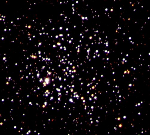
Here are our resulting pretty pictures. Click for a bigger image.
True-Color M11, in BVR
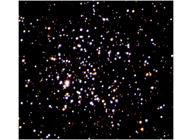
NGC 6819 in BVR
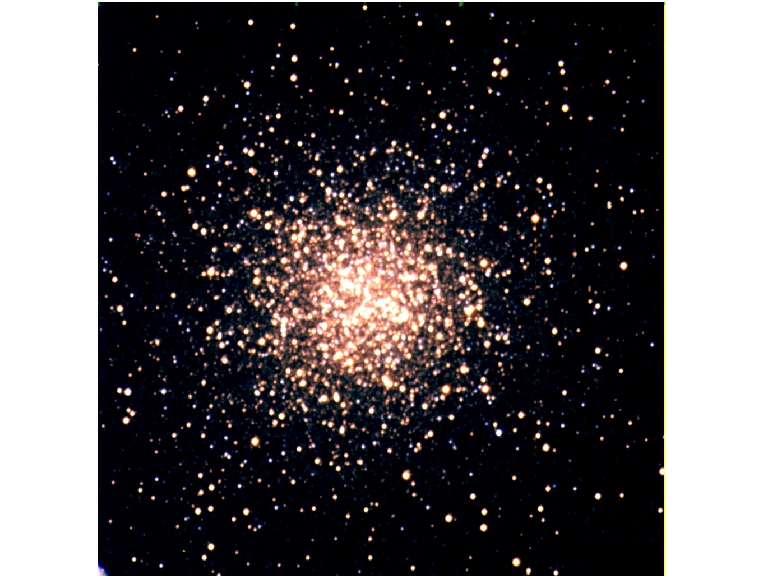
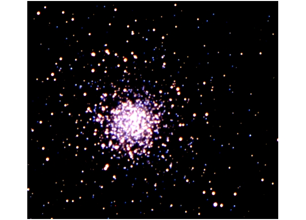
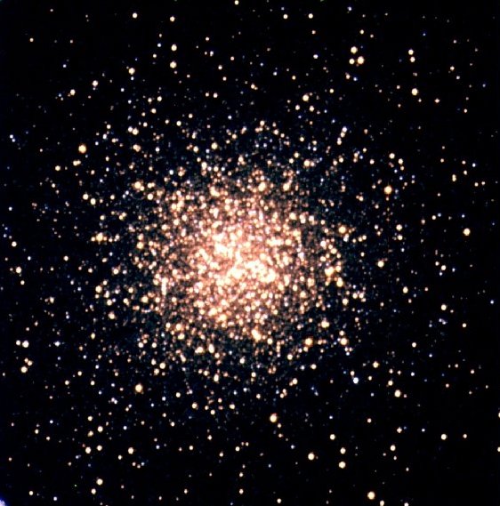
True-Color M13, in BVR
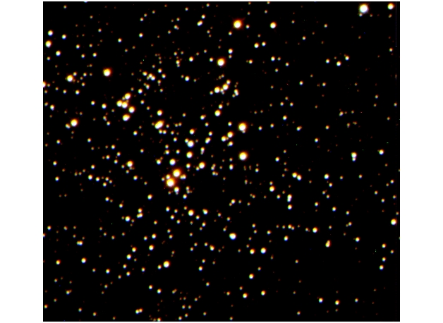
M5 in BVR

Data Reduction:
We decided to have our students brave the jungles of daophot. We used the stand-along version of Daophot for Mac OSX. We got this
software from Mike Bolte-- he might give it to you, too, if you take his class or ask nicely. The trickiest parts of this software were
a) finding enough Macs to run it on (we had to borrow our friends' powerbooks) and b) a 'daomaster' which has mysteriously stopped
working on Macs (we had to run this last step on a Linux machine).
Software you need installed on you Mac for this plan: DS9 or Ximtool, IRAF, and the daophot stand-alone software. You will also need our
macro script, which automatically runs all the daophot scripts and does lots of tedious iterations. It was originally developed by Katy
Flint, and was improved by Jenny Graves. It can be downloaded here as
"doall_phot". It should run if you copy it to the same directory as your images and daophot software, and make it executable.
You can download a pdf manual Laura wrote for our students here. It's not as detailed as she'd like it to be, but it's
hard to teach high schoolers about Mac and LINUX operating systems, IRAF, and photometry software all in one day. In theory,
students should only have to display their images, pick their PSF stars, run "doall_phot", and combine catalogs using
"daomatch" and "daomaster". This takes a whole day, though!!! Some of the students loved it. Maybe some of them hated it.
Tips:
1) We didn't realize how hard the concept of B-V would be for our students, and if we taught
this again, we'd spend longer on that.
2) We would suggest NOT combining multiple exposure in each filter, unless you really feel
like you are gaining critical sensitivity and/or dynamic range. It just takes way too long
and is very tedious.
3) Fix daomaster!!! If we did this again, I'd talk to Mike Bolte and get that thing fixed. I
wish I understood why it spontaneously broke. There seems to be no working version for Macs
right now.
When the students had their final allstar file, listing a magnitude for each star in B and V, we had them plot color-magnitude
diagrams in Excel. This worked well, but it was mostly for their instant gratification. The plots they used for isochrone
fitting were made by Kirsten and Laura in IDL. They can be seen below--Click for a larger image.
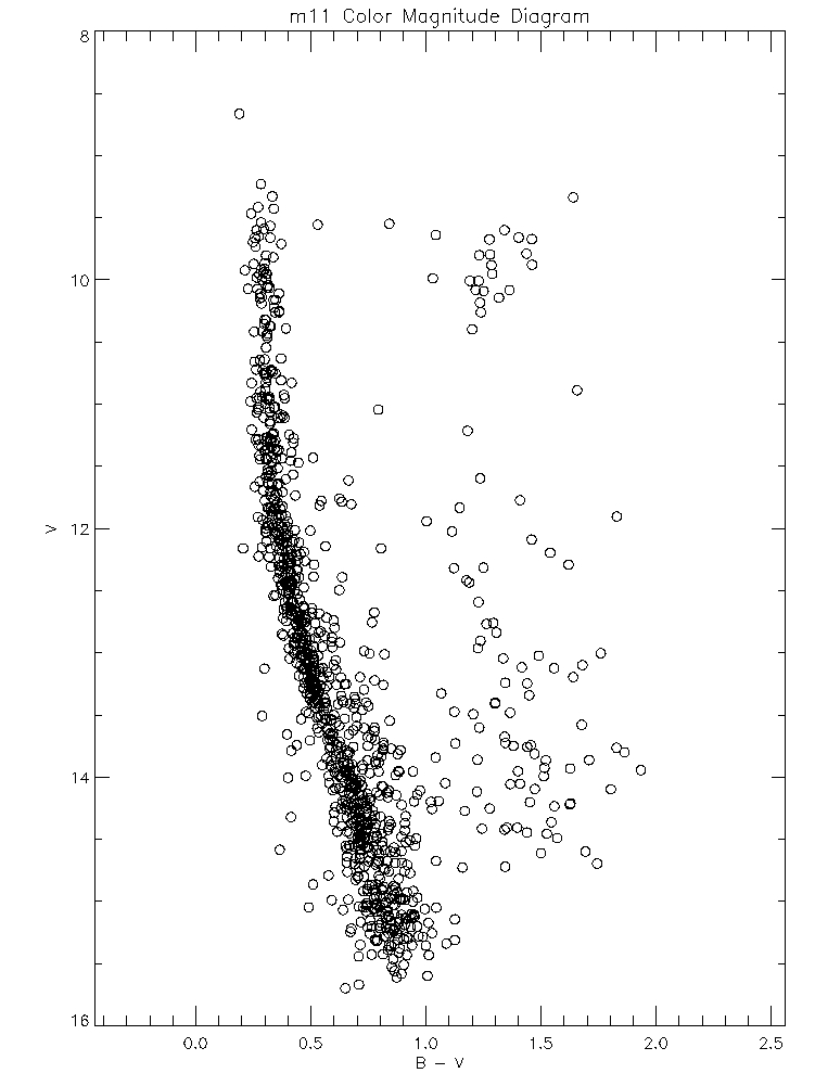
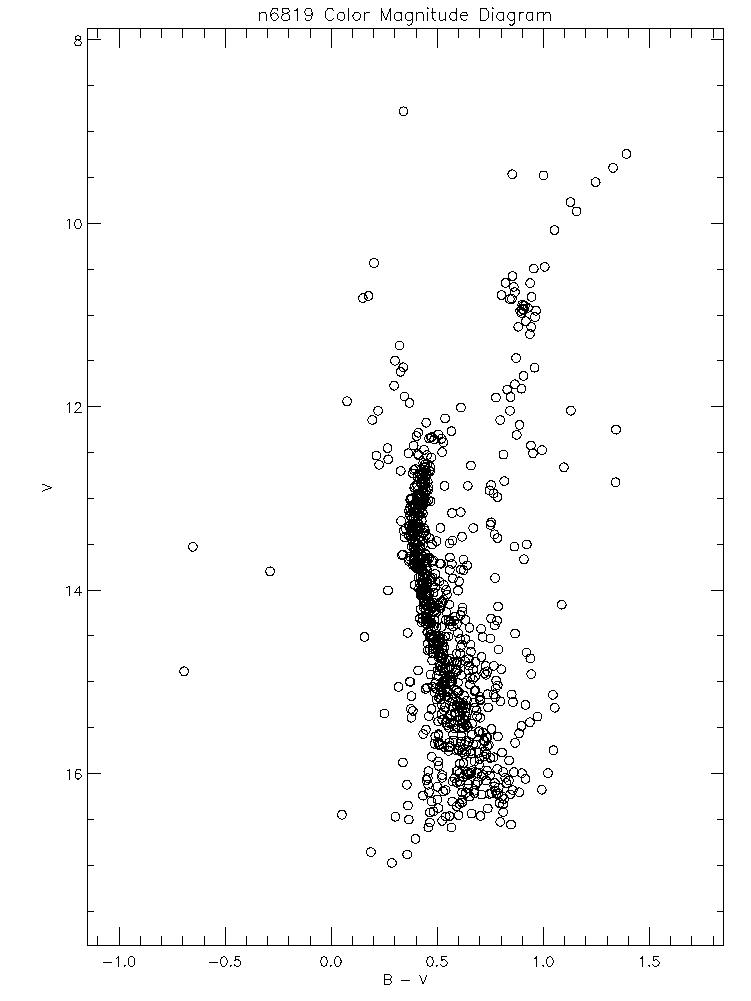
M11 Color Magnitude Diagram--Click for a larger image NGC
6819 CMD
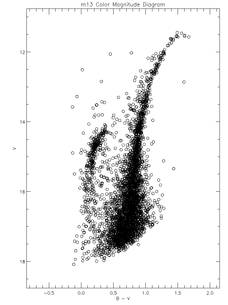
M13 Color Magnitude Diagram

Isochrone Fitting:
We used Yale Isochrones to find the ages of our clusters. We
printed out the isochrones to transparency film, making sure the isochrones had the right axes scales to match our cluster CMDs.
We printed out the whole age range for the students, from a tiny fraction a Gyr to 20 Gyr old.
Kirsten, do you want to include something about your IDL program???
***Make sure you use isochrones with the relevant metallicities for your cluster!!! We forgot to use sub-solar metallicities for
the globular clusters, so our students found their clusters to be 19 Gyr old!***
Then, simply have your students overlay the isochrones on their CMDs, and decide which fits best. This is a nice time for
collaboration and discussion.
Below is our students' isochrone fits for M11, NGC 6819, and M13. All isochrones were for solar metallicity.
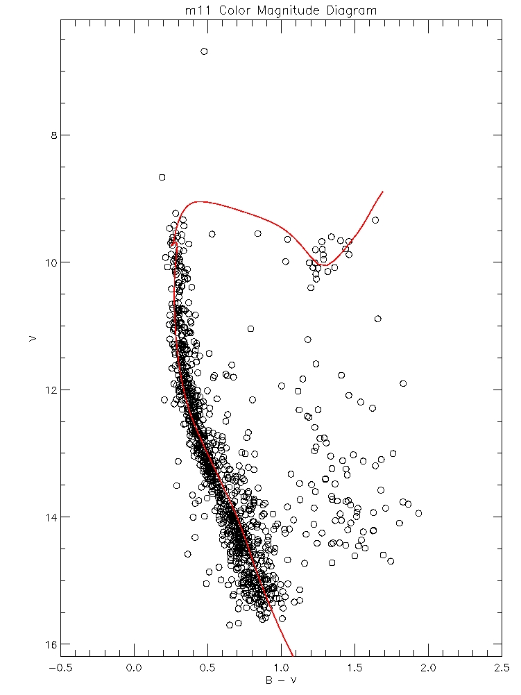
M11 CMD with 0.2 Gyr isochrone overlain
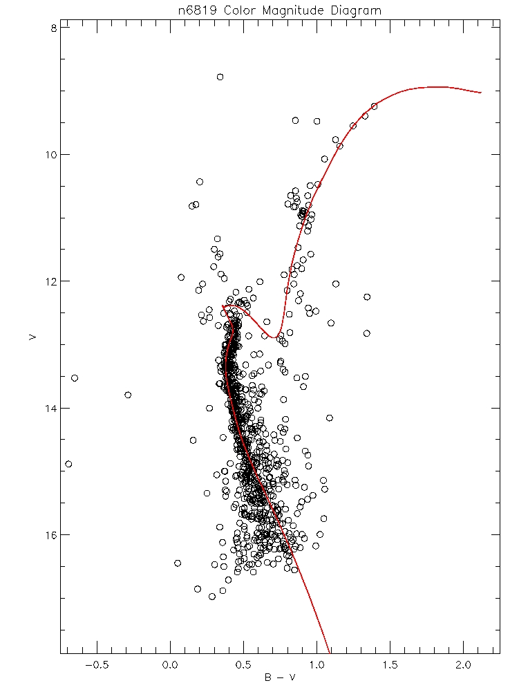
NGC 6819 CMD with 3 Gyr isochrone
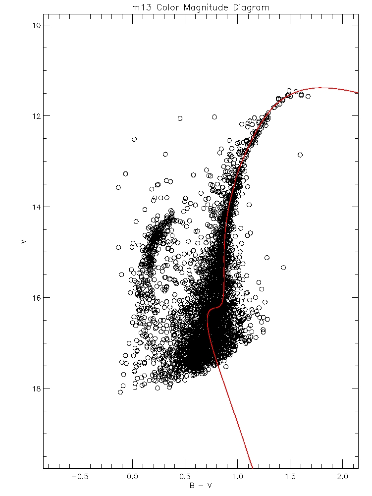
M13 CMD with 19 Gyr isochrone

Calculating Distances:
Now that our students had found good isochrone fits to their clusters, they "knew" the cluster absolute magnitudes from the
isochrone models. So all we had to do to get distances was callibrate our apparent magnitudes.
We've thought of two ways to callibrate the data, and we're not sure we have much faith in either. The first is a rather
pitiful excuse for a "method"-- we look up published CMDs of our clusters, and shift our observations' instrumental magnitudes
to fit the published apparent magnitude values. The second way is more scientific, and actually appeared to work ok this year:
we actually use standard stars and run daophot on them to get their brightnesses. The shift between the stars' "standard"
value and "our" value should be the same as the shift between our clusters' instrumental value and their true apparent value.
I think.
***We all know callibration is never as easy as it sounds. For goodness sake, see if it works and makes sense before trying to
callibrate in front of your students!!!***
We didn't do anything fancy like worry about reddening terms, or even about dust. We used the very simplest distance modulus
equation:
m - M = 5 log d - 5 with d in parsecs.
So, to recap, "M" comes from the isochrone models. "m" comes from your newly callibrated data. We shifted our isochrone
transparency around to match up with our CMD, and then looked at the difference between the two y-axes. That's "m-M"! Our
students did a bit of algebra (they knew logarithms pretty well) to extract the only unknown, "d".
Our results didn't match the best with published values-- especially for M13. Use sub-solar isochrones for globs!!! Also, um,
think about your calibration more than we did. If you wanted to be really hard-core, you could teach your students (and
yourself) about errors. Below are our measurements.
M11: 2600 pc
NGC 6819: 1400 pc
M13: 1000-3000 pc
As our students so astutely observed, But wait! I thought NGC 6819 was supposed to be farther away than M11! And M13 the
farthest of all! Our distances need help.
We tended to use the published distances for our galaxy models.

3-D Galaxy Models, to Scale:
Now that we know the distances to our star clusters, we can put them in the grander context of the Milky Way Galaxy. Kirsten
and Laura went to the Art Supply shop, the Lumber yard, and to their own closets to find the following supplies:
-- Large pieces of black foam board (for the galactic disk)
-- Assorted sizes of styrofoam balls (~8" diameter for a big galactic bulge. ~1" for a star cluster)
-- Red felt (to cover styrofoam balls for galactic bulges)
-- Pom Poms (multi-color)
-- X-acto Knives
-- Glue Gun
-- Lots of Glitter Glue (to make stars!)
-- Milky Pen (writes on Black board-- so students can label the Sun, etc.)
-- Dowels (two for each galaxy, each a bit longer than the disk's diameter)
-- Wire (for attaching the dowels together, and for hanging the galaxy and clusters from the dowels)
-- Wire cutters
We first talked about galactic features and scales. What is a bulge? How big is it? How far away from it are we? How long is
it from one end of the galaxy to the other? etc. We also talked about galactic coordinates, and had our students look up the
galactic coordinates for our clusters.
Some of our students chose to use the entire piece of foam board (~3' x 3') to make their galactic disks. However, we noticed
that there was no "to-scale" styrofoam bulge for a disk this size. So some of our students chose to be sticklers about scale,
and make smaller disks with to-scale bulges.
Our students cut their styrofoam bulges in half with kitchen or X-acto knives. Then they covered them in the felt, and glued
it on with the glue gun. They attached one half of the bulge to the center of foam board, and the other half to the underside
of the foam board.
Our students decorated their disks with the glitter glue and Milky Pen. They labelled the Sun's location and drew in spiral
arms.
Next, it was time to hang the galaxies. For each model, we took two dowels, and held them at right angles to each other, in
their centers, to make a cross. We tightly wrapped wire around their intersection, to hold them together. Then we cut four
pieces of wire, and our students made four holes evenly spaced in the outskirts of their disk. Each wire attached a corner of
their disk to a dowel. So the galaxies hung! We usually needed two people for this process. We also found that the galaxies
could be better observed if they were hung at some inclination. Finally, tie another piece of wire around the dowel
intersection, so that the galaxy can hang from the ceiling.
Finally, our students made four star clusters out of styrofoam balls or pom poms: two open clusters, and two globular
clusters. They attached these clusters in their correct places around the galaxy, given their galactic coordinates and
distances. For clusters which were far from the galactic plane, we attached the clusters to (stiff) wire, and had them
sticking up above the plane. I suppose that if the cluster was very high above the plane, it could dangle from the dowels. The
students labelled the clusters.
We really enjoyed this project, and we think our students did too. We had each student make their own model, which is nice,
but not necessary. The supplies can be a bit expensive. We'd probably allot 3-4 hours for this project, next time we did it.
Here are some photos of our students' lovely Milky Ways:


Catherine, Amanda, and Kirsten with their Galaxies
Molly and Becca with their Milky Ways (Jared not pictured here)

Our Students' Brilliant Presentations:
Our students worked really hard on their presentations, which they presented to their cluster-mates and the Robotics/Nanotech
Cluster. Download their powerpoint files below:
Globular Clusters
Open Clusters

Open Clusters in the Spotlight

Some General Conclusions:
We really liked having NGC 6819 there as an intermediate-age representative.
The Open Cluster group was able to deal with both M11 and NGC 6819. In the future, Open and Globular clusters could conceivably
be combined into one project. But that would mean no intermediate-age cluster, probably.
Kirsten, any final words of advice? Do you wanna mention submitting M5 to APOD?

Other Userful Links:
Scott Seagrove's write-up of his 2001 Globular Cluster Project,
including a great isochrone animation
Stuart Norton's Orignial Conception of this Project
CfAO COSMOS Page
Kathy Cooksey's 2005 COSMOS Page, including Observing Manual, etc.
Katy Flint's Help Page on Daophot, etc.


