Velocity dispersions from DEEP 2 1-d spectra

Ben Weiner 04/31/2003

This page compares emission-line velocity dispersions from DEEP2 first-season 1-d data, computed by two methods. The first is the dispersion produced by the Berkeley pipeline, through fitting of multiple broadened templates. The second is from automated fitting of Gaussians to individual emission lines, using a standalone program (referred to as "Santa Cruz" method strictly for convenience, not necessarily endorsed by others at UCSC).

The short story

Here's the comparison. There is clearly something going on that we need to understand.

Dispersion from Gaussian fit vs dispersion from pipeline template fit

Description of methods:

1. Berkeley pipeline: A template Vdisp.fits in log wavelength is made by setting delta functions at the locations of emission lines and convolving with a gaussian of sigma_inst approx 28 km/s to approximate instrumental resolution. A series of broadened templates are generated by convolving Vdisp.fits with gaussians of sigma = 0,10,...,400 km/s. Relative line intensities are held fixed and the velocity offset is assumed zero. The spectrum is shifted to restframe log wavelength and each template is fit to it, producing the run of chi-squared with sigma. A spline fit is used to find the minimum in chi-sq, and the error comes from a delta-chisq=1 criterion (I think).

This is from the procedures spec1d/pro/vdispfit.pro and findchi2min.pro. Corrections are welcome. This procedure uses the optimally-extracted spectrum.

2. "Santa Cruz" Gaussian fits: The program finds the expected locations of each of a short list of features and fits a Gaussian to each line. The fit to each line is independent. For the [O II] 3727 doublet, a double gaussian is fit and the line ratio is free to vary. The parameters for each line are continuum, intensity, velocity offset from nominal redshift, and dispersion. (Dispersions less than the instrumental are allowed, but rarely found in 4 sigma or greater detections.) The fit is a standard non-linear least squares routine, mrqmin from Numerical Recipes, and produces error estimates. For each object, if it had multiple lines I used the highest intensity line to get the dispersion. Only 4 sigma detections are used. The instrumental resolution assumed is sigma_inst = 0.63 A. (obtained by looking at SKYSIGMA from Berkeley pipeline v1_1 on a few masks). This used the boxcar-extracted spectrum.

Theoretical issue:

The treatment of instrumental resolution is not equivalent. Since DEIMOS is a grating spectrograph the resolution is basically constant in observed wavelength (unlike the SDSS spectrograph, I think). Using a constant siginst in restframe velocity of 28 km/s means a siginst in observed wavelength of (Wobs*28/c). This is 0.63 A at 6750 A. At longer Wobs, siginst is overestimated, so estimated velocity dispersion will be lower. However, this is only really significant for low intrinsic linewidths, under 50-60 km/s.

Practical issue:

When the two measures of linewidth are compared for a common set of objects, there are major differences, but they aren't all explained by the instrumental resolution issue.

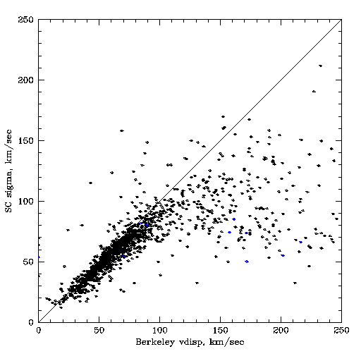
The plots below compare dispersions for a sample of galaxies with both dispersion estimates. The "Santa Cruz" dispersion comes from gaussian fits for objects in fields 2 and 3, v1_0 reductions, with 4 sigma detections. This list was matched to Berkeley dispersions from the file zcat.v1_0.fits. There were 1553 objects in the SC list, 1473 matches, 1265 had good Berkeley dispersions; the others presumably do not reach a minimum in chi-squared(sigma). Because the SC list is a subset, I did not count how many objects had a good Berkeley measure and a bad SC measure, but that is equally important.

Some results:

1. There are a number of objects for which the Berkeley dispersion is much higher than the SC dispersion. This is worst for high-dispersion objects and seems to affect nearly all objects with Berkeley disp above 100 km/sec.

2. There appears to be an offset in the sense that Berkeley disp is a little higher than SC. Could this be related to optimal versus boxcar extractions, or to splining the chi-squared(sigma) ?

3. There is a systematic difference trend with z. Perhaps related to optimal versus boxcar if relative weighting, window sizes and z are related? If so that is potentially a big issue. (There is the old airtovac wavelength issue, since these are v1_0 reductions, but it's hard to see how that could produce such a big difference.)

4. There appears to be a weak systematic difference with observed wavelength, in the expected direction. But they don't agree at 6750 A, due to the systematic offset.

5. Apart from the issues above the distribution of (Berkdisp - SCdisp) is basically consistent with the error estimates (plot not shown).

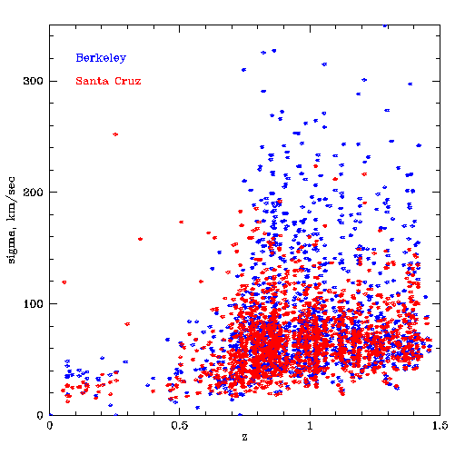
Dispersion vs redshift

Dispersion vs dispersion: high dispersion problem

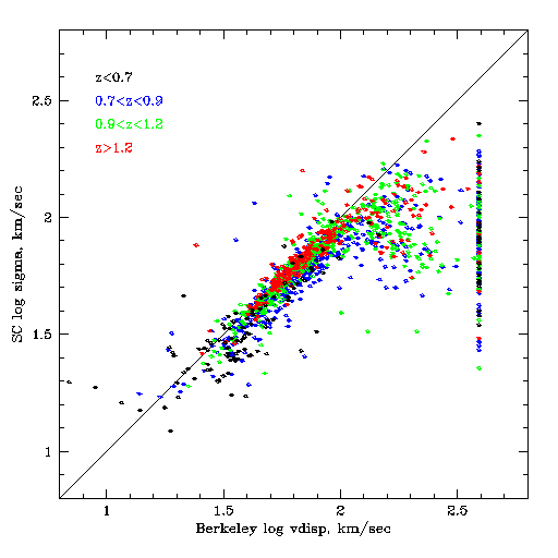
log dispersion vs log dispersion, colored by z range

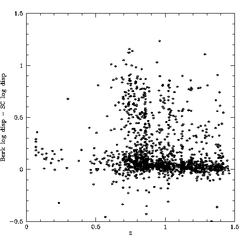
Difference in log dispersion, as function of z; trend with z

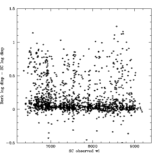
Difference in log dispersion, as function of observed wavelength; weak trend

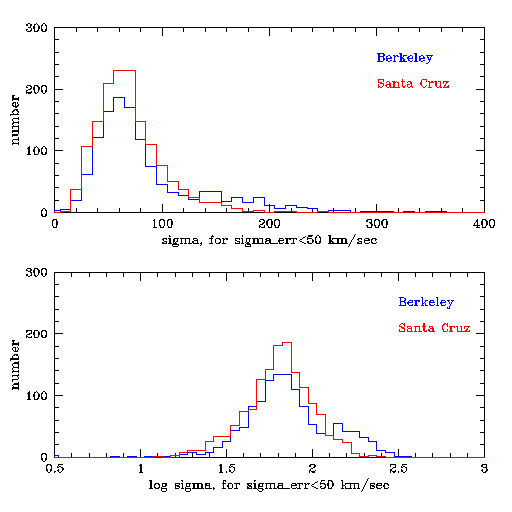
Histograms of dispersion

Sanity check

An obvious check is to see if the Gaussian fits are any good. The linefitting program produces GIF images of the data and fit around each line. Here are a few examples I looked at in the large-sigma disagreement regime. The Gaussians mostly look pretty reasonable, although there is one case where the fitting produces screwy results because it is not constrained to have a realistic ratio in the 3727 doublet.

mask.object     z     Bdisp   err   SCdisp  err  SC_line_used
2200.22016331  0.846  123.6  10.3    72.6   4.3   3728
2200.22031491  0.981  152.3   5.8   108.1   5.8   3728
2200.22031547  0.870  152.6   8.0    88.5   4.3   3728
2243.22060813  0.625  131.5   0.7    94.8   1.9   5007
2258.22025284  1.041  215    28.3    58.3   6.1   3728   low S/N
2280.22024423  0.827  183.3  15.3    94.6   9.7   3728
2280.22031928  1.057  152.3   5.5   169.8   5.8   3728   SC fit bad due to fitting a broad singlet to [O II], non gaussian lineshape
3202.32022827  0.743  130.3   2.4    80.4   2.8   5007

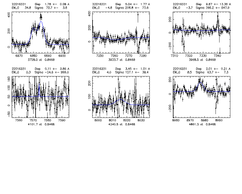2200.22016331

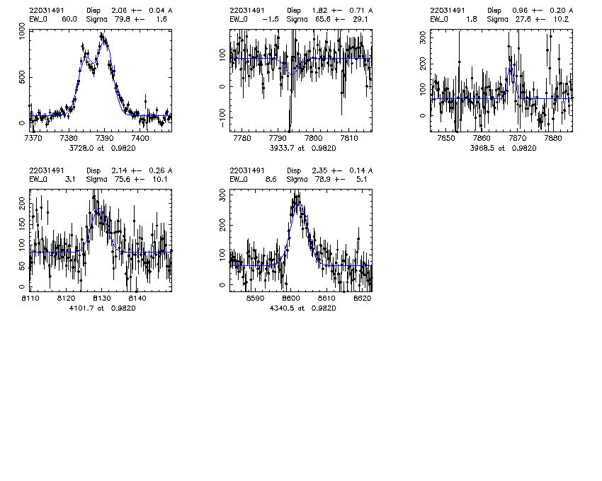2200.22031491

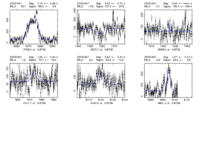2200.22031547

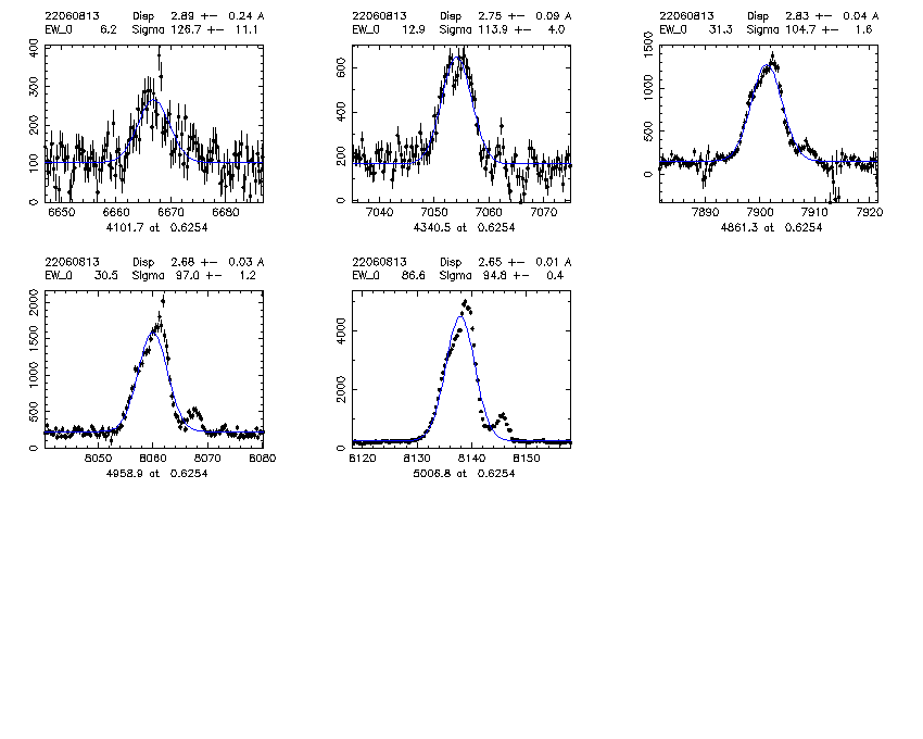2243.22060813

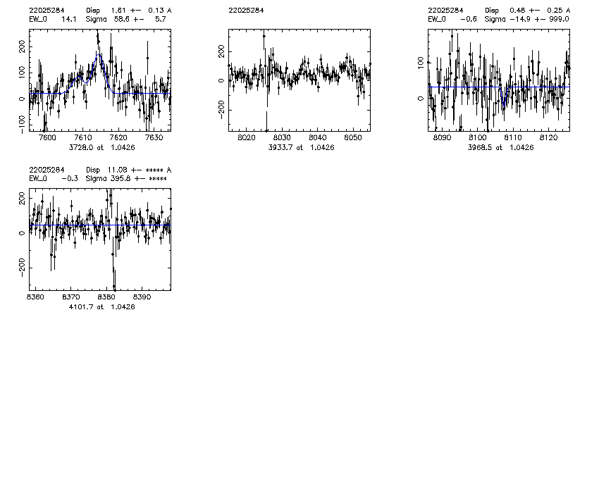2258.22025284

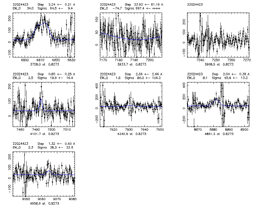2280.22024423

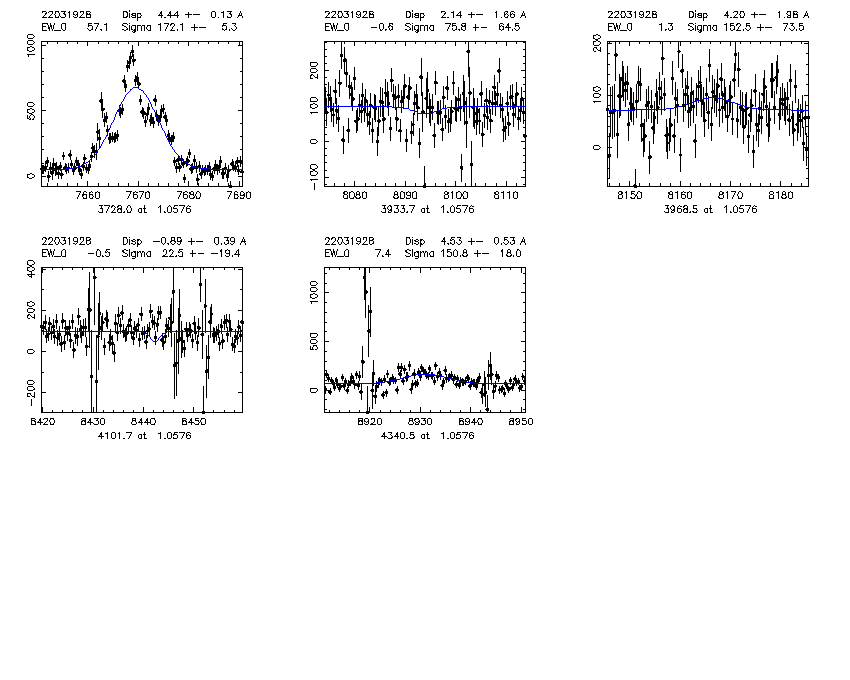2280.22031928 - bad fit, non Gaussian lineshape, more like the sum of two offset doublets

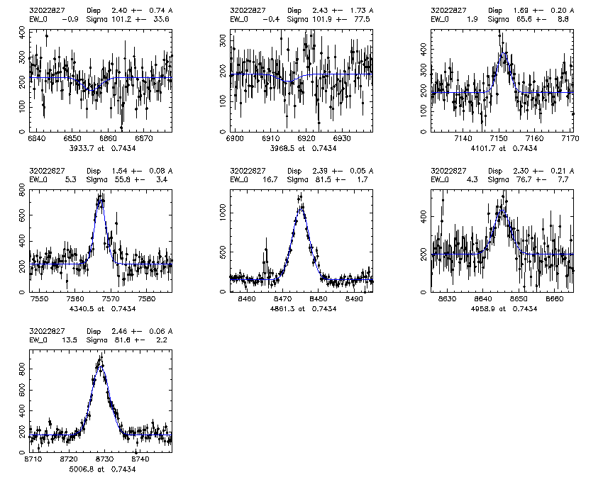3202.32022827

Science advertisement

Just to have some science content on this page, here is a plot showing the linewidth-magnitude relation and its evolution, in three redshift bins, using the Santa Cruz emission-line velocity dispersions described above. There is a Tully-Fisher relation at z=1 and it appears to be evolving. in slope and zeropoint.

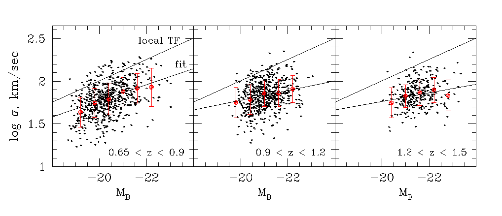
DEEP 2 linewidth-magnitude relation

Ben Weiner, 4/30/2003