2. The Camera Model
While much of the analysis could be analytical using geomtrical optics, in practice it was much easier to use a computer model of the camera and perform ray traces. This model was based on the ZEMAX model description of the 22C camera supplied by ORA. Its primary simplification is that it does not include any aspheric surfaces, but since our analysis applies to differential measurements, this should be quite adequate. The model includes 22 refractive surfaces (each characterized by an (x,y,z) location of the vertex, a radius of curvature, a thickness and an index of refraction) plus the CCD surface. The output showed the position and direction vectors for the intersection at each surface; inputs include the postion of the pinhole and angle of the test ray. In use, the angle was characterized by a single value (r1) which corresponds to the sine of the ray angle with respect to the optical axis.Example: dcam delx=0 r2=0 r1=0.02 (pinhole on-axis, angle=1.15 deg): (Surf Xmm Ymm Zmm r1 r2 r3) 1:x: 1.0002 0.0000 50.0008; r: 0.011481 0.000000 0.999934 2:x: 1.1446 0.0000 62.5751; r: 0.014115 0.000000 0.999900 3:x: 1.1458 0.0000 62.6615; r: 0.013784 0.000000 0.999905 4:x: 2.0225 0.0000 126.2587; r: 0.018804 0.000000 0.999823 5:x: 4.5123 0.0000 258.6449; r: 0.012204 0.000000 0.999926 6:x: 5.4730 0.0000 337.3590; r: 0.010430 0.000000 0.999946 7:x: 5.4997 0.0000 339.9119; r: -0.000301 0.000000 1.000000 8:x: 5.4968 0.0000 349.5611; r: 0.004617 0.000000 0.999989 9:x: 5.4981 0.0000 349.8421; r: 0.003869 0.000000 0.999993 10:x: 5.8717 0.0000 446.3934; r: 0.004120 0.000000 0.999992 11:x: 5.8720 0.0000 446.4772; r: 0.002738 0.000000 0.999996 12:x: 5.8983 0.0000 456.0860; r: 0.015955 0.000000 0.999873 13:x: 6.4463 0.0000 490.4279; r: 0.001863 0.000000 0.999998 14:x: 6.4637 0.0000 499.7328; r: 0.007672 0.000000 0.999971 15:x: 6.4643 0.0000 499.8218; r: 0.004824 0.000000 0.999988 16:x: 6.9268 0.0000 595.7017; r: -0.000585 0.000000 1.000000 17:x: 6.8897 0.0000 659.1201; r: -0.000585 0.000000 1.000000 18:x: 6.8862 0.0000 665.1191; r: -0.000585 0.000000 1.000000 19:x: 6.8714 0.0000 690.3928; r: 0.014141 -0.000000 0.999900 20:x: 6.9105 0.0000 693.1544; r: 0.033133 -0.000000 0.999451 21:x: 7.1279 0.0000 699.7109; r: 0.022712 -0.000000 0.999742 22:x: 7.4164 0.0000 712.4106; r: 0.033133 -0.000000 0.999451 IM x: 7.6388 0.0000 719.1210; r: 0.033133 -0.000000 0.999451 Thus, the ray falls at (x,y) = (7.64,0)mm on the CCD.
In the model, the pinhole was typically set 50mm in front of the first element (close to actual location) but the tests tend to be very insensitive to the exact distance. (The pinhole distance is actually at 0, with the first lens element at 50mm, as seen in the example above.)
Two tests were performed to verify the model. This first was simply to see if the plate scale was reasonable. The second was to see if on-axis collimated light was brought to a reasonable focus. This test required modelling an actual 6mm filter (assumed index = 1.545) and was run for 2 cases: a Back Focal Distance (BFD) of 0.2642in (Model B) and 0.287in (Model C).
 Radius at       Radius at       Radius at
 entrance        detector        detector
                  (Mod.B)         (Mod.C)
  .5mm            0.04 px        -0.01 px
   1mm            0.08 px        -0.03 px
   2mm            0.15 px        -0.05 px
   4mm            0.29 px        -0.12 px
   6mm            0.38 px        -0.23 px
   8mm            0.41 px        -0.39 px
  10mm            0.37 px        -0.63 px
  12mm            0.24 px        -0.97 px
  14mm           -0.01 px
  16mm           -0.41 px
  18mm           -0.95 px
  20mm           -1.67 px
Model C is near the BFD predicted by the 22C ORA model. Model B
gives a somewhat better focus across a larger-diameter input beam. The obvious
spherical aberration is no doubt due to the exclusion of aspheric terms
in the model. Nevertheless, Model B manages to focus a 32mm diam input
beam into less than 1 pixel.
Typical use:
for most of the analysis, the model was used on- or near-on-axis.
For example, the on-axis case produces a spot at (0,0)mm. Then an element
would be displaced by 0.1mm, and the on-axis input ray traced again, yielding
the amount of image motion at the detector. Finally, r1 would be adjusted so
that the ray passed through x=0.1mm at the lens surface; this would yield
the amount of shadow motion. For a few special cases, the model was run to
produce results at a specific location on the detector.
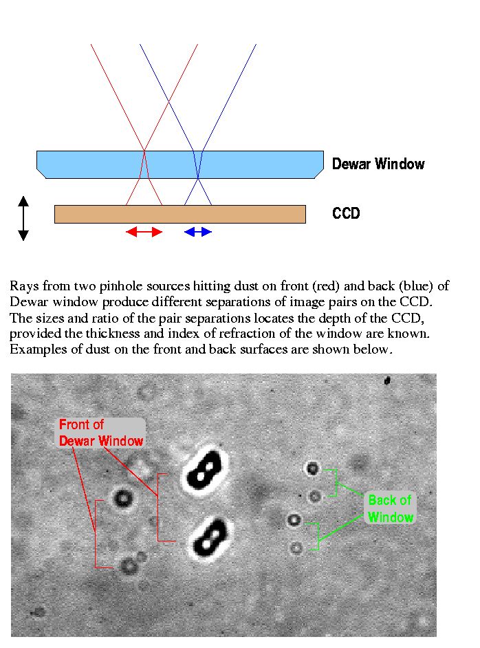
We have identified the following features with different separations:
On-axis results from Model A (which uses the 0C design camera, as the
ORA 22C model had not been received) state that dust/etc. on the front of the
Dewar window should cast shadows separated by 49px, while those on the back
of the window should cast shadows separated by 18px. This is close
to the 53-54px measured for the "[fairly-]sharp rings" and 23px measured
for the "very-sharp rings". Since the features are located so close to
the detector, this prediction is largely insensitive to the pinhole distance
in front of the camera, but it will be affected by the assumed distance
to the CCD (see next section). Also, note that there are no features seen
with separations less than 54 and 23 pixels, arguing that these will be
the 2 surfaces closest to the CCD.
The appearance of the condensation is that of "frost" at the edges
of the patch, and "ice" toward the center (as evidenced by linear light cusps).
There is also an obvious water droplet, whose edge casts images separated
by 54 px. This argues that the condensation consists of both liquid water
and ice.
See images of temporal changes also.
Thus we conclude that the bulk of the condensation is on the front
of the Dewar window. We cannot rule out some condensation in the center of
Element 9, since the condensation patch at the center of the window
is so large, but there is no direct evidence for it.
One frame (4243) was also taken at the back of the focus travel.
Quick measurements of the image separations on this image are 62 and 29 px.
This corresponds to a BFD of about 8.21mm +/- 0.4mm (0.3232in). Also, a
more sensitive test for the range of the focus stage (using the change in
plate scale across more than half the detector) yields a range of 1.9mm,
very close to the expected value.
The expected CCD distance, according to measurements provided by
Terry Pfister, is 0.2738in +/- 0.040in, or 5.94 to 7.97mm, behind the
Dewar window. These pinhole measurements indicate we are behind that
range by about 0.4mm.
An aside:
With Model D, we get a good match for all surfaces between the back
of Body 4 and the detector, as follows:
(After the camera flexure was identified (Section 4), a small
correction for the changing angle of the rays striking the CCD means that
the mosaic flexure should be slightly larger, by 0.14px, than determined here.)
To determine strongly moving features, images at different rotations
were "blinked" against each other; a few features were found that showed large
motions. (It was later found that dividing the images was a quicker way to
locate these features.) Three "spots" (rings), labelled A, B and C, were
strong enough to measure. Subsections around these spots were extracted
and shifted to remove the mosaic motion (that is, features on the Dewar
window were made stationary). Smaller subsections around each spot were
extracted, shifted and combined to form a template for each spot; the template
was also rotated 180 degrees so that cross-correlation would not pick up
any residual background features. Templates were then cross-correlated
against the individual images in order to measure motions.
Within each of the subsections above, it was noticed that the
relatively-common "diffuse rings" also had a slight motion. Therefore, a
region with several prominent "diffuse rings" was treated in a similar
manner to measure these motions. These features had been identified with
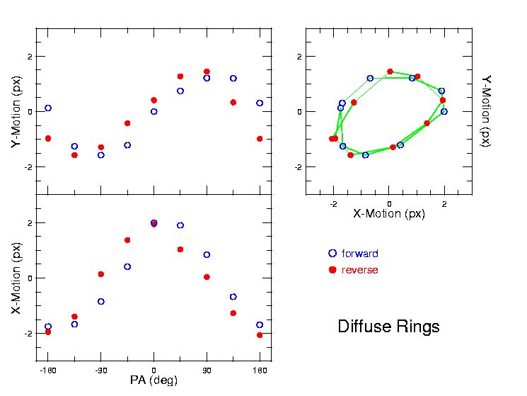
the back of Body 4 (Element 8), an identification confirmed below.
Description: tilted oval; 3.9 x 3.0 px (X x Y, FULL RANGE);
some hysteresis (perhaps 20-40 deg).
Body 4 is a POSITIVE doublet. Image motion will track element motion.
Y flexure should be maximum at PA=90;
X should be maximum at PA=0 if Body is moving under
gravity. This is observed. However, the optical model indicates a
shadow/image motion ratio of 3.4 ie, if Body 4 is moving, it is only
contributing about 1px of flexure (FULL RANGE). The observed shadow motion
implies about +/- 0.8 thou radial offset in Body 4.
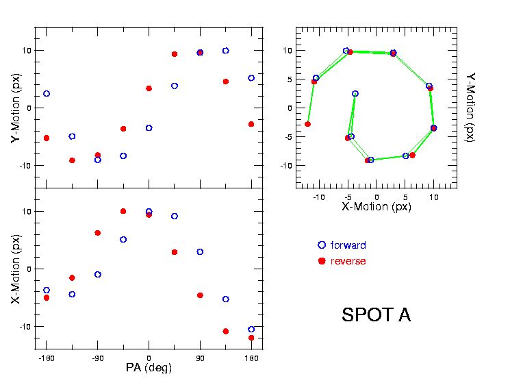
Oval helical pattern, closing with reverse rotation, dim 20x19 px;
hysteresis about 45 deg.
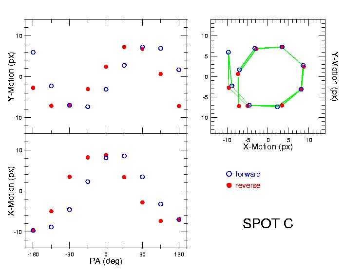
Oval helical, opening with reverse rotation, dim 18x14 px.
SPOTS A+C have similar size, appearance and (qualitatively) motion.
While XA-XC closes and reopens by 10px going from 180 to -180 to 180 again,
and YA-YC has similar results (by flipped in sign) the distance between these
spots is constant to within about +/- 1 px. Thus, this motion may well be
a rotation of Element 5. (del-y/del-x) varies from 1.296 to 1.304, a
difference of 0.17 deg. Therefore, Element 5 may be floating and
shifting by fairly large amounts, BUT the camera is insensitive to this
motion -- the ratio of shadow to image motion is 32:1. The observed
shadow motion implies a radial offset of +/- 4 thou.
Note that these spots may be due to bubbles in the coupling fluid
(a conclusion supported by the "soft" nature of their motion). However,
the phases indicate they follow gravity, which sounds contrary to what
bubbles would be expected to do.
The interpretation of these spots is uncertain, and we consider this
flexure term questionable.
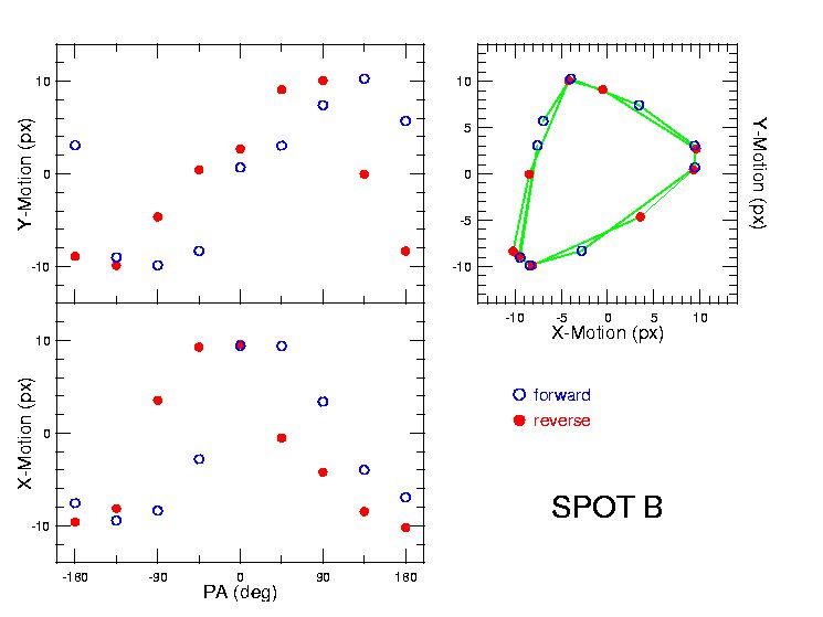
This loop closes, but is triangular in shape. There is about
45 deg hysteresis. Dimensions are 19x20, full range.
This spot is associated with the front of Element 3. The ratio of
shadow to image motion is 4.4:1, so that this motion is the dominant
contribution to camera flexure (4-5 px full range). The triangular shape
is consistent with the trifold symmetry of the elements supports.
Observed shadow motion implies a radial offset of +/- 2.7 thou.
NB: The spots associated with Elem 5 are likely to be bubbles in the
fluid couplant, and therefore may not represent actual element motion!!
Summary of motion:
1. The lens motions were worked out on a one-by-one basis and assumed
to add linearly. The assumption was verified by applying all of the motions
simultaneously in the model; the same net result was obtained.
2. Since we have a filter in place during normal operation, there is
the possibility that the presence of a filter might affect the shadow:image
motion ratios. Therefore, a set of model runs were made with the filter
in place and moving the elements radially as before. The ratios changed
negligibly:
3. The distance from the pinhole light source to the camera was
estimated to be 50mm, but was never measured precisely. The derived motion
most affected by this uncertainty would be that of Element 3, which is closest
to the light source. We thus derived the ratio of shadow:image motion
using a distance of 40mm instead; the ratio changed from 4.38 to 4.52.
Since a 20% change in distance produced only a 3% change in estimated
image motion, we conclude that this uncertainty is not very significant.
Displacing the camera elements as above produces slightly different
image motion across the image. With rays originating at the pupil (11.5in
in front of camera) we find:
In November 2000, we had identified 0.5px full range differential
flexure between points near +/- 54mm and points near +/- 6.6mm on the mosaic,
corresponding to r1 of 0.138 and 0.018, respectively. Predicted flexure over
this range would be +/- 0.40px (at r2=0.0393, appropriate for these
observations),
larger than what was seen by nearly a factor of 2. However, the camera flexure
may well have worsened over the past year if it is due to a shim slipping as
is hypothesized.
3. The Double Pinhole Test, Sept. 12
(Figure)
In the initial attempt to perform this test, the calibrated pinhole
(5 micron diam.) was held in place by two nylon screws, 18.8 mm apart; it
was not foreseen that the nylon would transmit light from the light source
behind. Thus, these images are dominated by light from 2 rather diffuse
sources 18.8mm apart. The images show a few very sharp features, many fairly
sharp features (including the central condensation patch), and some very
blurry images. Analysis (see section 3B) place the blurry features on
the field-flattener and on the window-glass filter which was in place
during these initial tests. Features in the images are generally "doubled"
with spacing of 53-54px for the numerous "fairly-sharp" features and 23px
for the less common "very-sharp" features (typical diameters of 12 and 17px,
respectively). The lower portion of the image is darker and only shows
one set of images, consistent with one of the light sources being occulted.
[The pinhole light source is held on the "camera mirror" spider, and the
occulting object is the mirror itself, located slightly to the side about
1 inch in front of the pinhole.]
  Feature:                  Obs. separation (pix)
  1. Very sharp rings             23
  2. Frost &c, sharp rings       53-54
  3. Dark rings                  84-94
  4. Dark blobs                   204
  5. Diffuse rings                468
Since only features very near the detector are usable, these data are not
useful for studying camera flexure. However, they may be used for three
ancillary studies: location of condensation, distance to CCD, and detector
motion.
A. Location of Condensation:
There are two likely spots for condensation to form: on the front
of the Dewar window, and on the front of the field flattener (Element 9).
Note that the space between Element 9 and the window is small and semi-sealed,
and that Element 9 is in thermal contact with the window at the edges.
The back of Element 9 is an unlikely location, since moisture will condense
onto the Dewar window instead. The front of Element 9 has been the
expected location, since the growth of condesation over time, and the current
amount of condensation, clearly requires a volume of air greater than the
space between Element 9 and the Dewar window.
B. Distance to CCD:
The lack of a truly close match in the results of the model above
(Model A) argues that the Back Focal Distance (BFD) is incorrect. Thus,
we can adjust the BFD to find a closer match. Model D (which incorporates
as closely as possible the exact setup used, including a filter), gives
the closest match at 54.2 and 22.7px for the front and back, respectively.
This model puts the CCD at a distance of 6.41mm (0.2524in) behind the Dewar
window. With potential measurement errors of 0.5px in each, the error
in distance is +/- 0.4mm.
   Feature:            Obs.sep.(pix)     Mod.D (on-axis)    Surface
  1. Very sharp rings      23              22.7           Back Dewar Win.
  2. Frost &c, sharp rings 53-54           54.2           Front Dewar Win
  3. Dark rings           84-94 (off axis) 80/86 on-axis  Bk/Front Elem9*
  4. Dark blobs           204             189/205         Bk/Frt Filter
  5. Diffuse rings        468              459            Back Elem 8

(*) Elem 9 is steeply curved, so image separation depends on both surface
(back/front) AND distance off-axis.
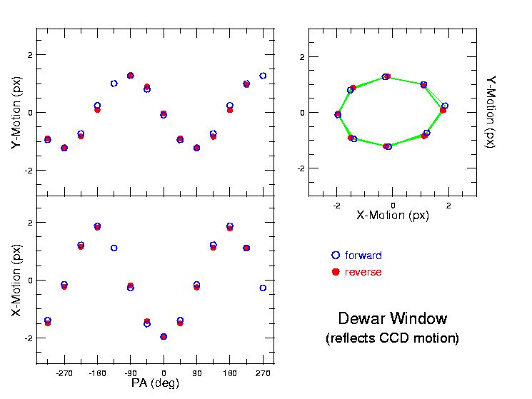
C. Detector Motion
We can use the apparent motion of the features on the Dewar window
to measure the flexure of the detector mosaic as DEIMOS is rotated.
The measurements were done by selecting some strong features, building an
averaged template, and cross-correlating. Results are that the detector
flexes in the direction of gravity by 1.8px (X) and 1.25px (Y). The motion
is very well behaved and there is only negligible hysteresis. [NB -- flexure
quoted is radius, thus full range of flexure is 3.8 x 2.5 px]
4. Camera Flexure Studies (Sept. 13, with followup Oct. 03)
Data collected on Sept. 13 had the nylon screws replaced with steel screws,
and a 100-micron pinhole in place. A full rotation sequence was obtained.
On Oct. 03, the pinhole was shifted slightly, to allow parallax measurements
to determine the exact location of features in the camera.
A. Location of Features
On Oct. 03, a pair of images was obtained with the pinhole
slightly shifted (with respect to the camera axis) between the exposures.
The shift was expected to be 1mm, but due to an error it was only a fraction
of this. Nevertheless, the data are usable (and the shift soluable). The table
below is separated into two parts -- the first is for on-axis parallax motion,
assuming a shift in the light source of 0.32mm, whereas the second is a
solution at the location of each of the measured features, with an adjusted
value for the pinhole shift of 0.30mm:
SURFACE		MODEL; .32mm	OBSERVED shifts		Feature observed
		On-Axis
Front Dewar:	  0.9 px	 < 1 px +/- <<1 px	ice in center
Surface 16:	  8.0 px	 6.7 px +/- 0.5 px	diffuse rings near SpotA
Elem 5/6:	 16.6 px	15.5 px +/- 0.5 px	Spot A ("moving spot")
Front Elem 3:    31.6 px	29.6 px +/- <1 px	Spot B ("moving spot")
Front of cam:	163   px	157. px +/- 2-3 px	Huge Spots F


FEATURE		MODEL; 0.3mm
		at feature
S16 near SPOT A:  6.8 px	 6.7 px +/- 0.5 px
SPOT A:		 15.6 px	15.5 px +/- 0.5 px
SPOT B:		 29.7 px	29.6 px +/- <1 px
SPOTS F:	154   px	157. px +/- 2-3 px
The agreement with specific features is remarkable.
B. Motion of Features and Moving Elements
(IMAGES)
As noted above, motion of different components was measured using
cross-correlation techniques. Next, the effect of displacing each element
was studied using the model, giving us the shadow motion produced by
a given offset, and the ratio of shadow motion to image motion.
By this technique, we can turn the shadow motion observed here into image
motion and determine how much a given element is displaced radially.
1. Diffuse Rings (Back of Body 4)
2. Spots A and C
3. Spot B
C. Camera Flexure Summary
We have identified motion associated with 3 optical elements:
In addition, we see motion of the mosaic by +/- 1.8 pixels (30% less in Y)
Elem 3:  +/- 2.7 thou ==> +/- 2.3 px image motion
Elem 5:  +/- 4   thou ==> +/- 0.3 px   (??) (somewhat less in Y)
Body 4:  +/- 0.8 thou ==> +/- 0.6 px   (25% less in Y)

Total:                    +/- 3.2 px

Detector (subtracts)      +/- 1.8 px   (30% less in Y)
                        ===============
                          +/- 1.4 px  Total image motion, Camera+detector
Note that the total flexure in the camera derived from shadow motions
is +/- 3.2 px, not quite the level of +/- 4.5 px expected from the COHU
observations. The difference between the two is not understood. (Possibly
there were some flexure in the COHU test setup?)
5. Miscellaneous Items
A. Possible Secondary Effects and Uncertainties
     Elem    Surfaces      Ratio w/o filt      Ratio w/ filt
       3        5/6             4.38                4.41
       5        9/10           32                  32
      7+8      13/16            3.37                3.42
B. Distortion (Differential Flexure)
        r1     Theta   Del-x_(mm)  rel_to_0.0551mm
      -0.16     -9.2     0.0550        0.0001
      -0.14     -8.0     0.0529        0.0022
      -0.12     -6.9     0.0510        0.0041
      -0.10     -5.7     0.0495        0.0056
      -0.08     -4.6     0.0485        0.0066
      -0.06     -3.4     0.0475        0.0076
      -0.04     -2.3     0.0470        0.0081
      -0.02     -1.1     0.0467        0.0084
       0	 0       0.0466        0.0085
       0.02      1.1     0.0466        0.0085
       0.04      2.3     0.0470        0.0081
       0.06      3.4     0.0476        0.0075
       0.08      4.6     0.0484        0.0067
       0.10      5.7     0.0497        0.0054
       0.12      6.9     0.0509        0.0042
       0.14      8.0     0.0529        0.0022
       0.16      9.2     0.0553       -0.0002
Thus, we see that with flexure compensation at the edges of the mosaic, the
camera flexure would still produce an image motion of +/- 0.0085mm or
+/- 0.57px at the center of the detector. Failure to fix the camera flexure
would thus degrade image quality.
C. Image Motion Caused by Filter
Most of the data collected on Sept. 13 had the filter removed from
the optical train, but the final exposure (4320) had the science filter
inserted for direct comparison with the previous frame (4319). It was
found that images of features in front of the filter shifted by about
7 pixels toward lower X (image coordinates). This raised the issue of
whether the filter might be contributing to flexure. However, subsequent
tests using the FCS and applying pressure to the filter wheel in various
directions did not produce any image motion, so it seems likely that
the observed shift in images is due to wedge in the filter.