Contents:

Comparison
Optimization
   Aggressiveness
   Track Time

Site Conditions
Image Processing
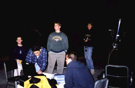
Binary Stars

These experiments are intended for students at several educational levels.  The goals of the experiments get increasingly more ambitious. The basic ones are designed for high-school and undergraduate students. The advanced ones may be more appropriate for graduate students.  This is not meant to restrict the experiments students should try, but may serve as a guide for the laboratory instructor.

Before trying the experiments, it is expected that students have read the introductions to the telescope and the tip-tilt camera, and are familiar with the instruction manual. Laboratory instructors should either be familiar with observing with small telescopes, or receive training from the Center for Adaptive Optics (CfAO). The overall goal of the experiments is to have students gain experience with each aspect of the system, and develop enough confidence to make their own scientific observations using adaptive optics (AO). For each experiment we outline a potential method, and give some comments on what worked for us.

The AO Demonstrator team observing at Mt. Hamilton:
Left to right are Robert Cook, Jarrett Kodani, Eric Steinbring, Gary Creason, and Lisa Hunter. Brian Lemaux is taking the picture. The 0.25 meter telescope and tip-tilt system is at far right. It is portable, and with practice, fairly easy to operate. In this picture, we have set up next to the dome of the 3 meter telescope at Lick Observatory, and Jarrett and Gary are analyzing images of binary stars.

Purpose: Determine the improvement in image quality with AO correction.

Point to a very bright star (roughly 0th magnitude) which is roughly straight overhead. When you place it in the tracking charge-coupled device (CCD) it should provide at least a couple of stars on the imaging CCD. Take a  guided and unguided exposure using this guide star. Do the AO-on and AO-off images look different?  NOTE: Make sure that the stars are in both exposures. 

Using the camera software, CCDOPS, the full-width at half maximum (FWHM) of a star can be determined from an image. This is done by selecting the Display Menu and then the Show Crosshair command. The crosshair window will appear and the arrow will then change to a crosshair symbol when placed on the image. When the crosshair is placed over a star, two numbers will appear, like 4.8 by 7.3, in the Seeing value of the Magnitudes box in the crosshair window. The first number is the FWHM in the X-axis, while the second number is the FWHM in the Y-axis. Left click on the mouse button and a small box will appear. Continue pressing the "t" key on the keyboard until the box is as big as the star. This box will determine the size of the area sampled to find the FWHM.

Give the stars in your image designation numbers. Determine either the X or Y FWHM of the stars for each exposure.  Make a bar graph of AO-on and AO-off FWHM for each star and compare. Did AO improve the images and if not, why? (Hint:  What is the value of aggressiveness?)

Our Experiment: We took a non-AO (Figure 1.1) and AO exposure (Figure 1.2) of a star field while guiding on the star Vega.  We then determined the X FWHM for the four stars of each exposure.  We made a bar graph of the data (Graph 1.1).  It seems that the AO correction made the stellar images sharper, but some more than others. Can you think why the measurements are not all exactly the same?

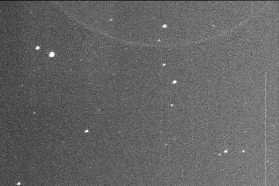Figure 1.1: AO-off image.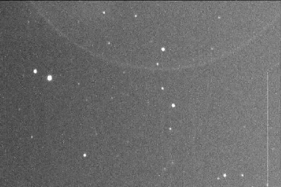



Figure 1.2: AO-on image.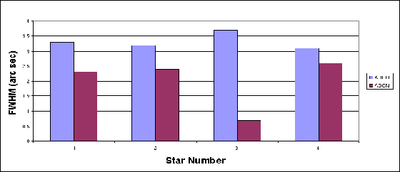



Graph 1.1: Comparison between AO-off and AO-on.

Contents

Purpose: Determine the aggressiveness setting that produces a minimum FWHM.

In CCDOPS, the value of aggressiveness is how much the mirror moves for each corrective step. The default value is 10. An aggressiveness of 20 would move the mirror twice as much as a value of 10. Try to select a value that will best suppress the wander (given in units of arcseconds) of the star displayed in the Guiding Dialogue. You can tell if the aggressiveness is too high when the star begins to oscillate a lot. The most probable best values will be between 5 and 15 but, as with everything, play with it until an optimum is found. (The aggressiveness can be adjusted during guiding by hitting the "+" and "-" keys.). At what aggressiveness does the star begin to oscillate wildly?

Find a very bright guide star which provides at least one star on the imaging CCD. First, take an unguided exposure. Then take an AO exposure of the star with the aggressiveness at 1. Continue taking AO exposures while increasing the aggressiveness by one until an aggressiveness of 20 is reached.

Determine the either the X or Y FWHM of the star for each exposure. Make one plot of the FWHM versus aggressiveness for all 20 exposures. The optimum aggressiveness should have a minimum FWHM. Can you find a minimum FWHM?

Our Experiment: We again used Vega as our guide star. We took exposures while increasing the gain from 1 to 20. We then determined the average FWHM of the star for each exposure. We made a plot of the FWHM versus aggressiveness for all 20 exposures (Graph 2.1). The optimal aggressiveness was found to be between 6 and 14.  This value gave images with a FWHM of about 3 arcseconds, an improvement of about 30% over no correction.  Is your improvement similar?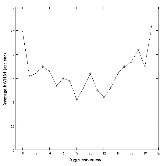

Graph 2.1: Average FWHM versus aggressiveness.

In CCDOPS, the track time is the exposure time for the tracking CCD. The minimum value is 0.001 seconds. This is how long it takes the tracking CCD to take a picture.  The computer and tip-tilt mirror also require a finite amount of time to respond, so each cycle will actually take longer to complete. 

Find a bright guide star which provides at least one star on the imaging CCD. Take an AO exposure of the star with the track time at 0.001 seconds. Continue taking AO exposures while increasing the track time by ten intervals until a track time of 10 seconds is reached.

Give each star a designation number. Determine the either the X or Y FWHM of the star for each exposure. Make one plot of the FWHM versus track time for all 10 exposures. The optimum track time should have a minimum FWHM.

Our Experiment: Again using Vega as a guide star, we took exposures at several different track times between 0.001 to 10 seconds. We then determined the average FWHM of the star for each exposure. We made a plot of the FWHM versus the logarithm of track time for all exposures.  Unfortunately, vibrations in the floor of the roof shook our telescope and overwhelmed the abilities of the AO system. We need to try this experiment again. 



Contents

Purpose: Determine the effect of site conditions on AO corrected images.

There are several external variables which reduce the effectiveness of correction. The most obvious are wind, and heat rising from warm surfaces.  By controlling these factors, the resolution should be improved.  This can be done by putting up wind shields or changing observing sites, for example.

Choose a factor to control, like wind conditions, and then a means of control, like changing locations.  Perhaps you could try the roof of a building or an open field. How about in a sheltered location, away from the wind? Where do you expect the air to be less turbulent?  At the first observing site, find a guide star which, when placed on the tracking CCD, has a star on the imaging CCD.  Take an AO exposure of the star.  Change the site location and repeat the process using the optimal aggressiveness and track time.

Determine the X or Y FWHM of the stars for each exposure.  Make a bar graph of the FWHM for each site and compare. Were some sites better than others?  Would the results be better if you were to take the telescope to a mountain top? Why?

Our Experiment: We took exposures at four different sites using Vega as a guide star.  The first two sites were beside and on top of the astronomy building on the Santa Cruz campus (at see level). The second two sites were at Lick Observatory on Mt. Hamilton (elevation of about 1300 meters). We determined the X FWHM for a star in each exposure and made a bar graph of the data (Graph 4.1). The best site was 4, the second site on Mt Hamilton.  Now, it is true that these observations were made on different nights, which may have had some effect, but it still seems Mt. Hamilton provides better results than the campus.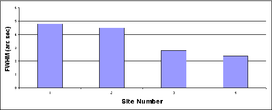

Graph 4.1: Comparison of optimal FWHM for four sites.

Purpose: Process AO-corrected images to see if they can be further improved.

Raw images from the camera have defects, but there are remedies which you can apply:

1. Bias Signal.  This is extraneous signal coming from the camera amplifier and electronics.  This is usually negligible, but reading out the camera after exposing for 0 seconds will measure the effect. Subtracting this bias frame from the image will correct for it.
2. Dark Current.  Heat from the camera causes the detector to register more photons than there should be. This results in a spurious signal, or dark current. A dark frame is an exposure with the shutter closed. You then subtract the dark frame from the image.
3. Sensitivity Variations. Each pixel of the CCD has a slightly different sensitivity to photons. This sensitivity bias can be corrected by dividing by a flat field.  A flat field is an exposure of a uniform background, such as the sky at twilight.
4. Sky Background.    The night sky has some illumination even though it looks dark to the eye. This signal is subtracted from the image.  This is done by finding the mean brightness of all the pixels in the image and then subtracting it from each pixel. 
5. Deconvolution.  For many reasons, flaws in the stellar image may exist. It may not be round, or it may be blurry, or there may be a slight flare on one side. By assuming the light from a star should have a specific shape - that of a sharply focused point source - a deconvolution algorithm is able correct the image. Often this dramatically improves the quality of images, however, applying too much deconvolution can produce unwanted artifacts and increase the noise in the image. There is deconvolution software provided in the software package. It is called CCD Sharp.

Find a bright guide star which provides at least one star on the imaging CCD. Take an AO exposure of the star field. Take a dark frame. Take a flat field.

Determine either the X or Y FWHM of the star in the unprocessed exposure.  Complete each of the post processing steps and look at the images.  Do they look better? You should be able to see fainter objects, but does the FWHM improve?

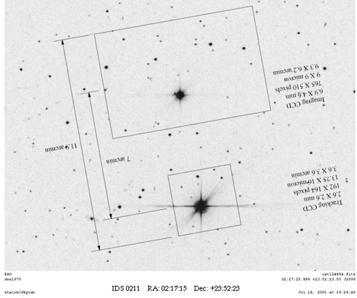
Our Experiment: We used Vega as a guide star and selected the auto contrast feature to do sky subtraction (Figure 5.1).  We had already taken a flat field exposure of the evening sky (Figure 5.2).  We also took a dark current exposure (Figure 5.3). We applied flat field division (Figure 5.4) and dark current subtraction (Figure 5.5). Finally, we used the deconvolution feature in CCD Sharp (Figure 5.6).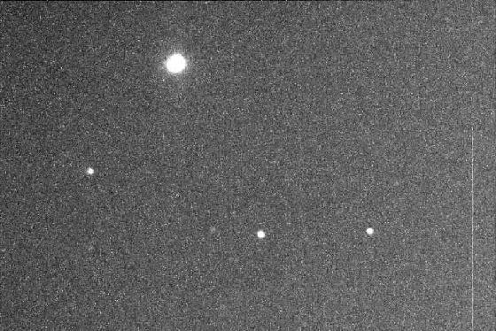

Figure 5.1: Original image.



Figure 5.2: Flat field.



Figure 5.3: Dark field.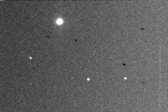



Figure 5.4: Flat-fielded image.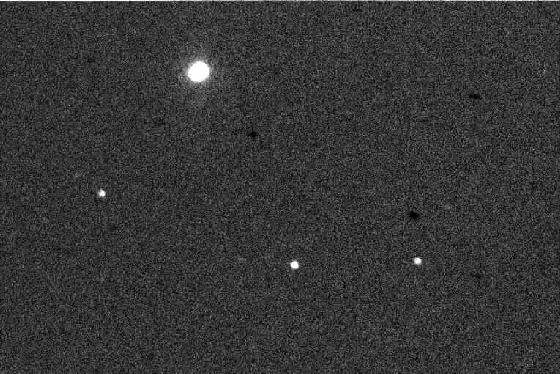



Figure 5.5: Dark-subtracted image.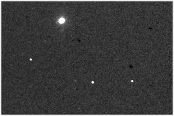



Figure 5.6: Deconvolved image.

Purpose: Observe binary star systems and attempt to resolve the individual components.

Binary star systems consist of two stars orbiting around each other. Most appear very close together on the sky and are difficult to resolve without AO.  Post processing may also improve the results.

Find a binary star system in which a nearby 7th magnitude or brighter guide star can be placed on the tracking CCD. A list of potential targets, with separations of 1 to 5 arcseconds are provided in Table 6.1.  Finder maps of the surrounding sky are provided as well.  They have the same scale as the diagram of the CCD camera provided in the manual Appendix. You'll need to orient the camera to get the guide star on the guide detector and the binary in the imager.  There are tips for doing this in the manual.  It takes some practice, so be patient.  (Hint: Figure 6.0 shows the correct orientation for the binary IDS 0211.) Take an non-AO and AO exposure of the system.

Determine the X and Y FWHM of the stars for each exposure. Determine the average FWHM of the stars in both. Note the difference between both exposures. Did you resolve the two stars? Does post processing the image help?

Table 6.1:  Visual binaries with guide stars suitable for the AO Demonstrator 

Name	s (")	vA	vB	R.A. (2000)	Dec. (2000 )	vgs	r (')	p.a.	finder
IDS 02117N2325	4.80	8.22	8.51	02:17:15.74	+23:52:24.8	6.59	6.46	191
IDS 04012N5000	1.62	8.49	9.87	04:08:42.09	+50:16:23.2	7.00	4.44	169
IDS 04046N4136	1.08	9.25	9.29	04:11:27.01	+41:51:35.5	7.00	7.21	201
IDS 05369N2519	2.64	8.42	9.47	05:43:03.21	+25:21:48.2	6.80	9.30	61
IDS 05525N6458	1.80	8.89	10.85	06:02:21.49	+64:58:06.0	6.69	5.72	344
IDS 10124N2801	4.57	8.01	9.14	10:18:05.54	+27:31:27.9	5.97	6.66	170
IDS 11517N4055	1.57	8.72	10.32	11:56:53.87	+40:21:21.6	6.59	4.03	101
IDS 12120N7042	2.14	9.28	9.54	12:16:47.12	+70:08:45.8	5.69	8.97	291
IDS 12430N0400	4.29	8.02	10.85	12:48:04.02	+03:27:19.1	6.40	7.71	336
IDS 13418N4132	2.31	7.58	9.87	13:46:02.78	+41:02:16.1	5.80	3.67	34
IDS 18344N2837	1.12	8.56	9.19	18:38:22.45	+28:41:49.3	6.59	6.37	231
IDS 18480N1353	1.42	8.72	8.74	18:52:35.03	+14:00:12.2	6.19	8.34	254
IDS 20092N1551	1.21	8.28	8.35	20:13:44.93	+16:09:28.6	6.37	6.87	339
IDS 20438N2705	1.10	8.63	9.14	20:48:06.26	+27:27:25.6	5.67	8.87	340
IDS 20507N3219	1.11	8.06	8.10	20:54:49.88	+32:42:23.1	6.75	7.24	98

     Name:  The binary's designation in the IDS catalog.
     s:  The separation between the two components in arcseconds.
     vA:  The visual magnitude of the A component star.
     vB:  The visual magnitude of the B component star.
     RA and Dec:  The right assention and declination of the binary.
     vgs:  The visual magnitude of the guide star.
     r:  The separation between the binary and the guide star in arcminutes.
     p.a.:  The position angle of the guide star relative to the binary, measured from the western horizon.
     finder:  The link to the finder chart for the surrounding area in .pdf format. The star in 
              the center of the finder is the binary.

Our Experiment: We took an exposure of binary star system IDS 0211 (Figure 6.0 and Figure 6.1). We then performed image processing procedures to resolve the stars even further (Figure 6.2). This is the most widely separated binary from our list and so it was fairly easy to resolve the two stars.  For future work we could take pictures over an extended period (months to years) and map the orbit of one star about the other.  Why would we want to do this?

Figure 6.0: The IDS 0211 field with the CCD field-of-view diagram overlaid.

Figure 6.1: Original image of binary IDS 0211.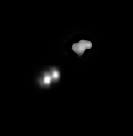

Figure 6.2: Processed binary image showing the peaks of the stars (lower left). The unguided image is shown for comparison (upper right).